class: center, middle, inverse, title-slide # STA 517 3.0 Programming and Statistical Computing with R ## Reshaping Data ### Dr Thiyanga Talagala --- # Data Wrangling/ Data Munging  -- # Reshaping Data (tidying your data) How to reshape your data in order to make the analysis easier. --- # Tidy Data 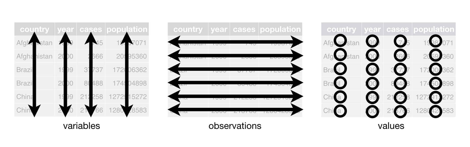 - Each variable is saved in its column. - Each observation is saved in its own row. .footer-note[.tiny[.green[Image Credit: ][Hadley Wickham and Garrett Grolemund](https://r4ds.had.co.nz/tidy-data.html)]] --- # packages ```r library(tidyverse) #or library(tidyr) library(magrittr) ```   --- # `tidyr` package Hadley Wickham, Chief Scientist at RStudio explaining tidyr at WOMBAT organized by Monash University, Australia. <img src="tidyr/tidyrhadley.JPG" alt="knitrhex" width="550"/> Image taken by [Thiyanga S Talagala](https://thiyanga.netlify.app/) at WOMBAT Melbourne, Australia, December-2019 --- 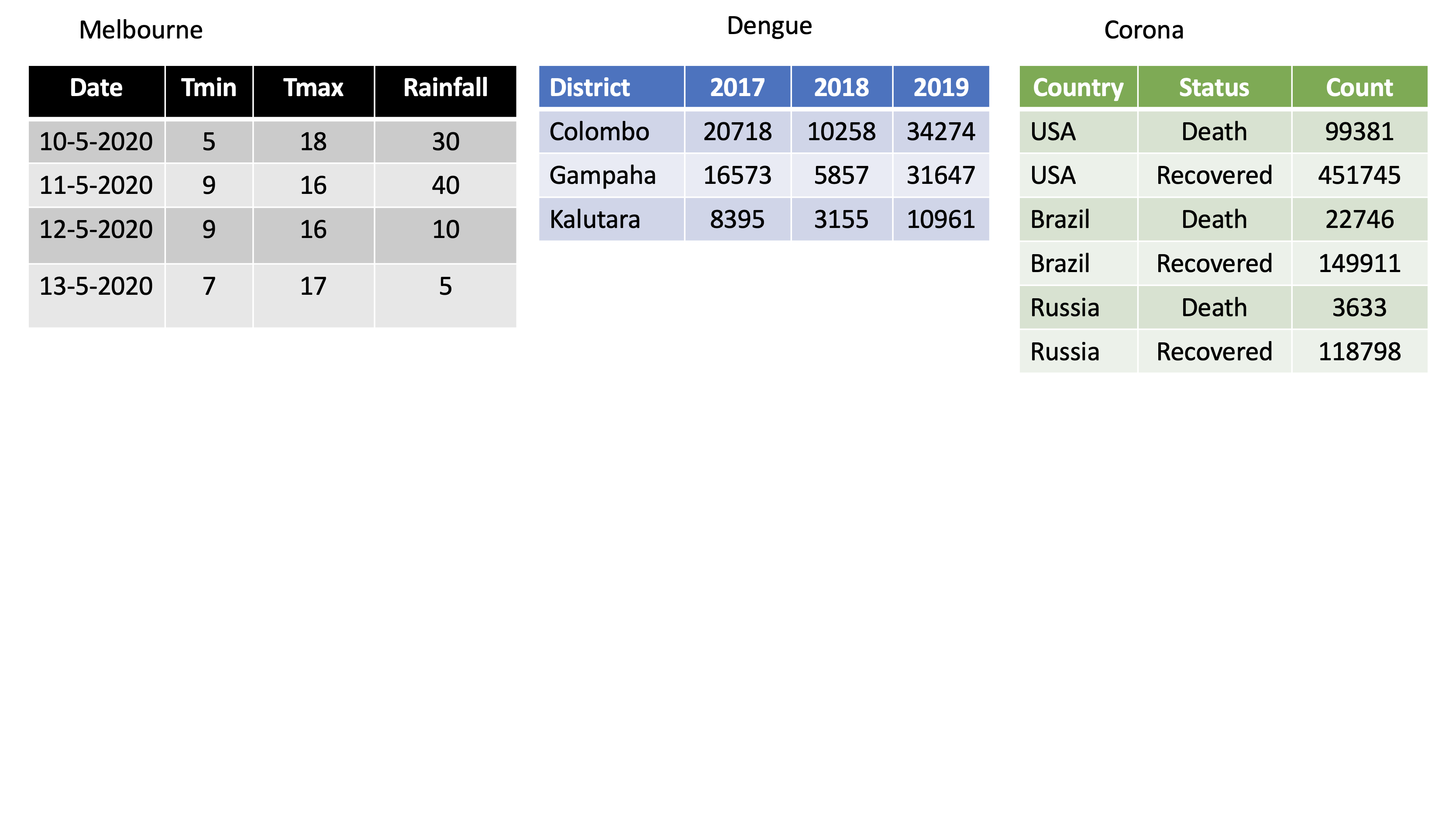 --- 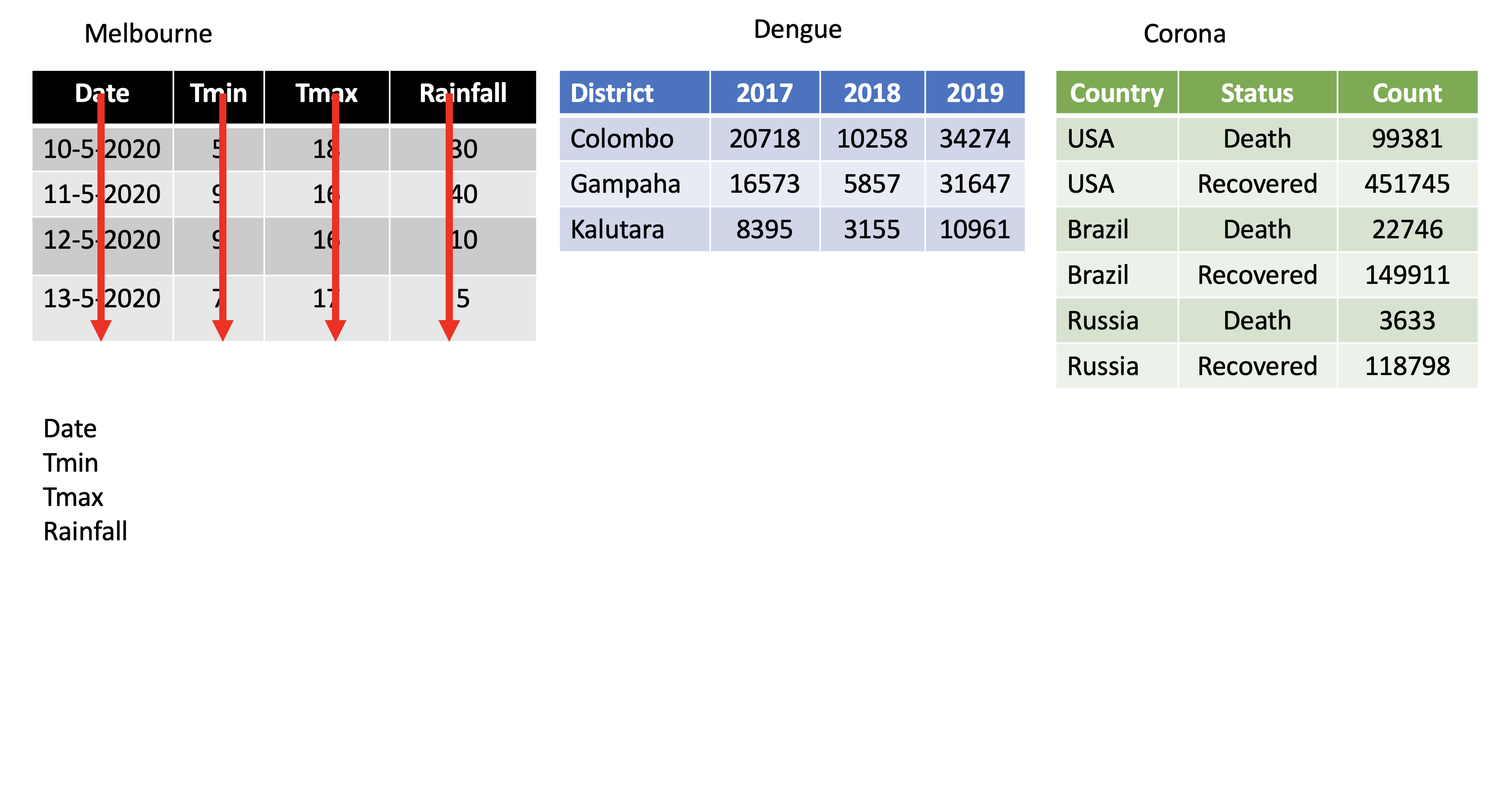 --- 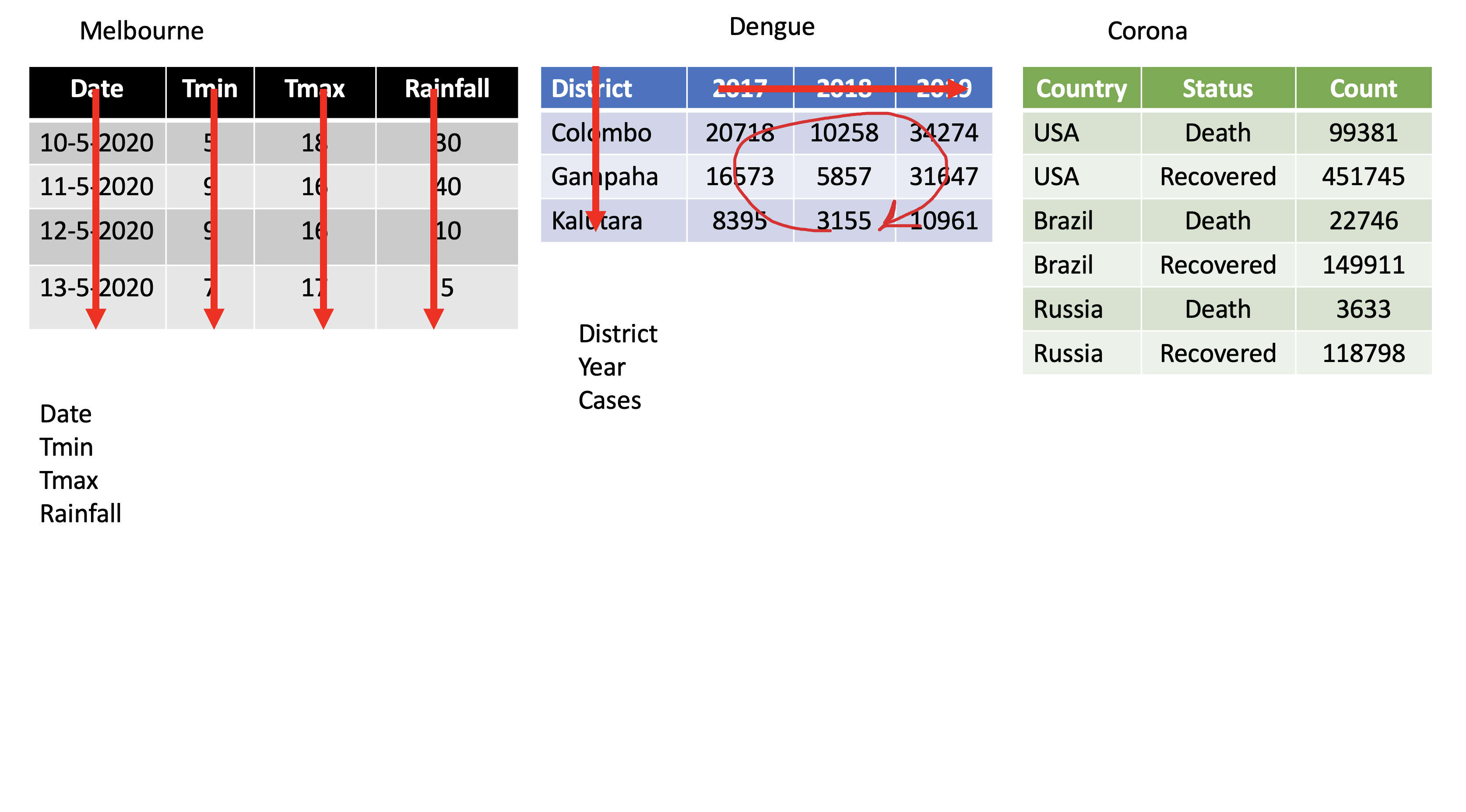 ---  ---  --- background-image: url(tidyr.jpeg) background-size: 100px background-position: 98% 6% # tidyr verbs ## Main verbs - `pivot_longer` In tidyr (2014) `gather` - `pivot_wider` In tidyr (2014) `spread` ## Other - `separate` - `unite` ## Input and Output Main input: `data frame` or `tibble`. Output: `tibble` --- class: duke-orange, center, middle # `pivot_longer` --- # `pivot_longer()` - Turns columns into rows. - From wide format to long format. 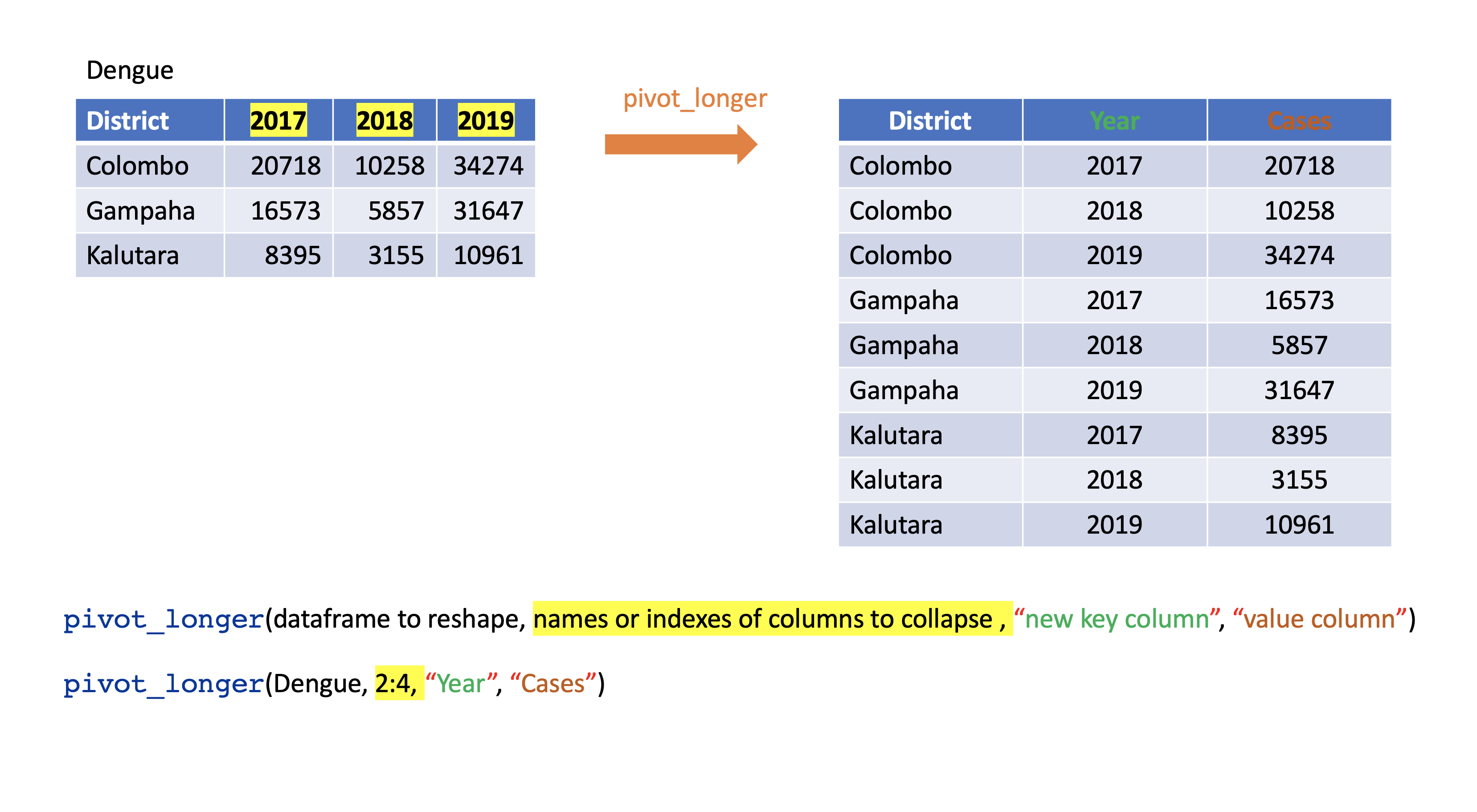 --- ## `pivot_longer()` ```r dengue <- tibble( dist = c("Colombo", "Gampaha", "Kalutara"), '2017' = c(20718, 10258, 34274), '2018' = c(16573, 5857, 31647), '2019' = c(8395, 3155, 10961)); dengue ``` ``` # A tibble: 3 × 4 dist `2017` `2018` `2019` <chr> <dbl> <dbl> <dbl> 1 Colombo 20718 16573 8395 2 Gampaha 10258 5857 3155 3 Kalutara 34274 31647 10961 ``` ```r dengue %>% pivot_longer(2:4, names_to="Year", values_to = "Dengue counts") ``` ``` # A tibble: 9 × 3 dist Year `Dengue counts` <chr> <chr> <dbl> 1 Colombo 2017 20718 2 Colombo 2018 16573 3 Colombo 2019 8395 4 Gampaha 2017 10258 5 Gampaha 2018 5857 6 Gampaha 2019 3155 7 Kalutara 2017 34274 8 Kalutara 2018 31647 9 Kalutara 2019 10961 ``` --- class: duke-orange, center, middle # `pivot_wider` --- # `pivot_wider()` - From long to wide format. 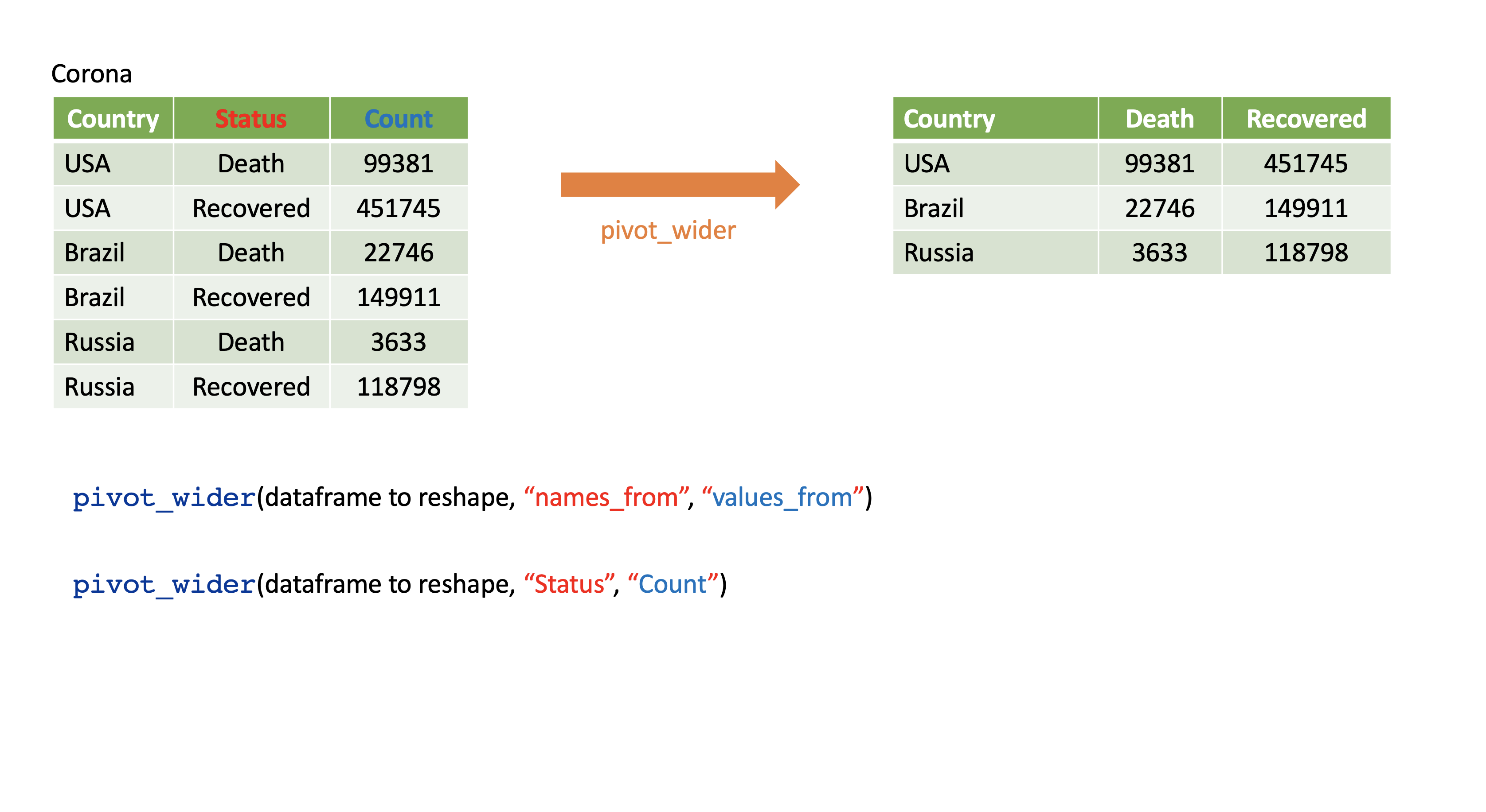 --- # `pivot_wider()` ```r Corona <- tibble( country = rep(c("USA", "Brazil", "Russia"), each=2), status = rep(c("Death", "Recovered"), 3), count = c(99381, 451745, 22746, 149911, 3633, 118798)) ``` ```r Corona ``` ``` # A tibble: 6 × 3 country status count <chr> <chr> <dbl> 1 USA Death 99381 2 USA Recovered 451745 3 Brazil Death 22746 4 Brazil Recovered 149911 5 Russia Death 3633 6 Russia Recovered 118798 ``` --- # `pivot_wider()` .pull-left[ ```r Corona ``` ``` # A tibble: 6 × 3 country status count <chr> <chr> <dbl> 1 USA Death 99381 2 USA Recovered 451745 3 Brazil Death 22746 4 Brazil Recovered 149911 5 Russia Death 3633 6 Russia Recovered 118798 ``` ] .pull-right[ ```r Corona %>% pivot_wider(names_from=status, values_from=count) ``` ``` # A tibble: 3 × 3 country Death Recovered <chr> <dbl> <dbl> 1 USA 99381 451745 2 Brazil 22746 149911 3 Russia 3633 118798 ``` ] --- # Assign a name: ```r *corona_wide_format <- Corona %>% pivot_wider(names_from=status, values_from=count) *corona_wide_format ``` ``` # A tibble: 3 × 3 country Death Recovered <chr> <dbl> <dbl> 1 USA 99381 451745 2 Brazil 22746 149911 3 Russia 3633 118798 ``` --- # `pivot_longer` vs `pivot_wider` 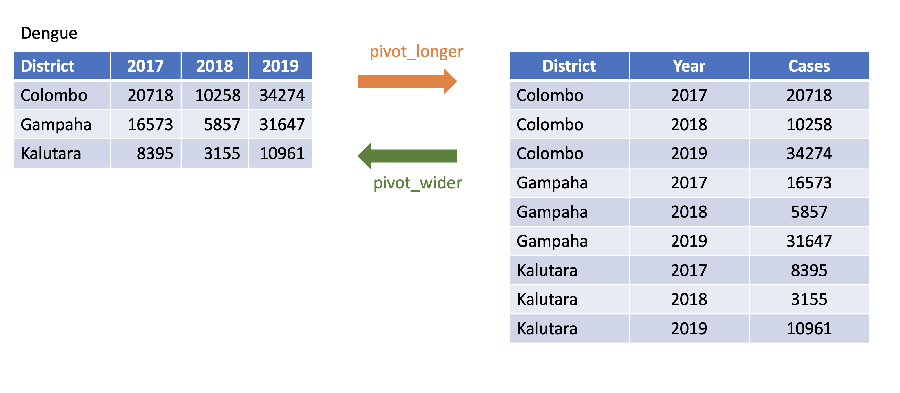 --- # `pivot_longer` and `pivot_wider` ```r profit <- tibble( year = c(2015, 2015, 2015, 2015, 2016, 2016, 2016), quarter = c( 1, 2, 3, 4, 2, 3, 4), income = c(2, NA, 3, NA, 4, 5, 6) ) profit ``` ``` # A tibble: 7 × 3 year quarter income <dbl> <dbl> <dbl> 1 2015 1 2 2 2015 2 NA 3 2015 3 3 4 2015 4 NA 5 2016 2 4 6 2016 3 5 7 2016 4 6 ``` --- # `pivot_longer` and `pivot_wider` ``` # A tibble: 7 × 3 year quarter income <dbl> <dbl> <dbl> 1 2015 1 2 2 2015 2 NA 3 2015 3 3 4 2015 4 NA 5 2016 2 4 6 2016 3 5 7 2016 4 6 ``` ```r profit %>% pivot_wider(names_from = year, values_from = income) ``` ``` # A tibble: 4 × 3 quarter `2015` `2016` <dbl> <dbl> <dbl> 1 1 2 NA 2 2 NA 4 3 3 3 5 4 4 NA 6 ``` --- # Missing values ``` # A tibble: 4 × 3 quarter `2015` `2016` <dbl> <dbl> <dbl> 1 1 2 NA 2 2 NA 4 3 3 3 5 4 4 NA 6 ``` ```r profit %>% pivot_wider(names_from = year, values_from = income) %>% *pivot_longer( *cols = c(`2015`, `2016`), *names_to = "year", *values_to = "income", *values_drop_na = TRUE ) ``` ``` # A tibble: 5 × 3 quarter year income <dbl> <chr> <dbl> 1 1 2015 2 2 2 2016 4 3 3 2015 3 4 3 2016 5 5 4 2016 6 ``` --- class: duke-orange, center, middle # `separate` --- # `separate()` - Separate one column into several columns. ```r Melbourne <- tibble(Date = c("10-5-2020", "11-5-2020", "12-5-2020","13-5-2020"), Tmin = c(5, 9, 9, 7), Tmax = c(18, 16, 16, 17), Rainfall= c(30, 40, 10, 5)); Melbourne ``` ``` # A tibble: 4 × 4 Date Tmin Tmax Rainfall <chr> <dbl> <dbl> <dbl> 1 10-5-2020 5 18 30 2 11-5-2020 9 16 40 3 12-5-2020 9 16 10 4 13-5-2020 7 17 5 ``` ```r Melbourne %>% separate(Date, into=c("day", "month", "year"), sep="-") ``` ``` # A tibble: 4 × 6 day month year Tmin Tmax Rainfall <chr> <chr> <chr> <dbl> <dbl> <dbl> 1 10 5 2020 5 18 30 2 11 5 2020 9 16 40 3 12 5 2020 9 16 10 4 13 5 2020 7 17 5 ``` --- # `separate()` ```r df <- data.frame(x = c(NA, "a.b", "a.d", "b.c")) df ``` ``` x 1 <NA> 2 a.b 3 a.d 4 b.c ``` ```r df %>% separate(x, c("Text1", "Text2")) ``` ``` Text1 Text2 1 <NA> <NA> 2 a b 3 a d 4 b c ``` --- # `separate()` ```r tbl <- tibble(input = c("a", "a b", "a-b c", NA)); tbl ``` ``` # A tibble: 4 × 1 input <chr> 1 a 2 a b 3 a-b c 4 <NA> ``` -- ```r tbl %>% separate(input, c("Input1", "Input2")) ``` ``` ## Warning: Expected 2 pieces. Additional pieces discarded in 1 rows [3]. ``` ``` ## Warning: Expected 2 pieces. Missing pieces filled with `NA` in 1 rows [1]. ``` ``` ## # A tibble: 4 × 2 ## Input1 Input2 ## <chr> <chr> ## 1 a <NA> ## 2 a b ## 3 a b ## 4 <NA> <NA> ``` --- # `separate()` ```r tbl <- tibble(input = c("a", "a b", "a-b c", NA)); tbl ``` ``` # A tibble: 4 × 1 input <chr> 1 a 2 a b 3 a-b c 4 <NA> ``` -- ```r tbl %>% separate(input, *c("Input1", "Input2", "Input3")) ``` ```r tbl %>% separate(input, c("Input1", "Input2", "Input3")) ``` ``` ## Warning: Expected 3 pieces. Missing pieces filled with `NA` in 2 rows [1, 2]. ``` ``` ## # A tibble: 4 × 3 ## Input1 Input2 Input3 ## <chr> <chr> <chr> ## 1 a <NA> <NA> ## 2 a b <NA> ## 3 a b c ## 4 <NA> <NA> <NA> ``` --- class: duke-orange, center, middle # `unite` --- # `unite()` - Unite several columns into one. ```r projects <- tibble( Country = c("USA", "USA", "AUS", "AUS"), State = c("LA", "CO", "VIC", "NSW"), Cost = c(1000, 11000, 20000,30000) ) projects ``` ``` # A tibble: 4 × 3 Country State Cost <chr> <chr> <dbl> 1 USA LA 1000 2 USA CO 11000 3 AUS VIC 20000 4 AUS NSW 30000 ``` ```r projects %>% unite("Location", c("State", "Country")) ``` ``` # A tibble: 4 × 2 Location Cost <chr> <dbl> 1 LA_USA 1000 2 CO_USA 11000 3 VIC_AUS 20000 4 NSW_AUS 30000 ``` --- # `unite()` ```r projects %>% unite("Location", c("State", "Country")) ``` ``` # A tibble: 4 × 2 Location Cost <chr> <dbl> 1 LA_USA 1000 2 CO_USA 11000 3 VIC_AUS 20000 4 NSW_AUS 30000 ``` ```r projects %>% unite("Location", c("State", "Country"), * sep="-") ``` ``` # A tibble: 4 × 2 Location Cost <chr> <dbl> 1 LA-USA 1000 2 CO-USA 11000 3 VIC-AUS 20000 4 NSW-AUS 30000 ``` --- # `separate` vs `unite` 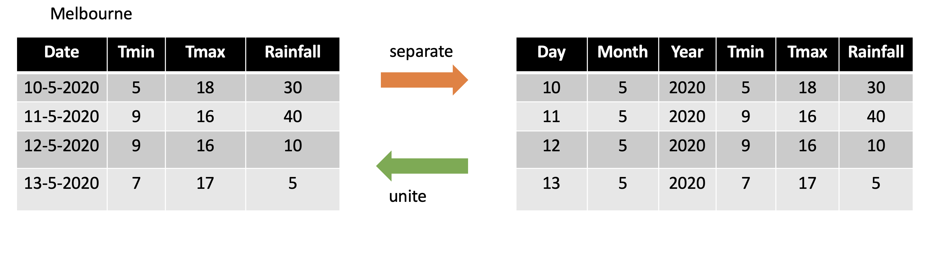 --- class: center, middle Slides available at: hellor.netlify.app All rights reserved by [Thiyanga S. Talagala](https://thiyanga.netlify.com/)