class: center, middle, inverse, title-slide # STA 326 2.0 Programming and Data Analysis with R ## Introduction to the tidyverse ### Dr Thiyanga Talagala ### Online distance learning/teaching materials during the COVID-19 outbreak. --- background-image: url(stayhome.jpg) background-position: center background-size: contain --- background-image: url(tidyverse.jpeg) background-size: 100px background-position: 98% 6% # What is the tidyverse? - Collection of essential R packages for data science. - All packages share a common design philosophy, grammar, and data structures. ### Setup ```r install.packages("tidyverse") # install tidyverse packages library(tidyverse) # load tidyverse packages ``` 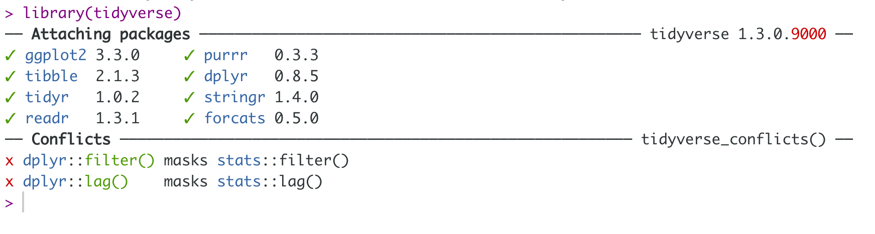  --- background-image: url(workflowds.png) background-position: center background-size: contain # Workflow .footer-note[.tiny[.green[Image Credit: ][Wickham](https://clasticdetritus.com/2013/01/10/creating-data-plots-with-r/)]] --- background-image: url(readr.png) background-size: 100px background-position: 98% 6% # Workflow: import 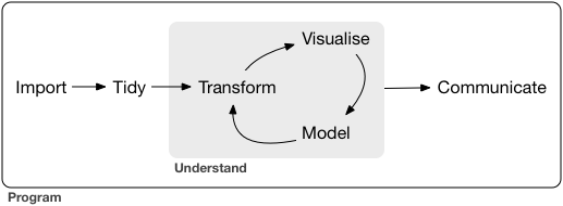 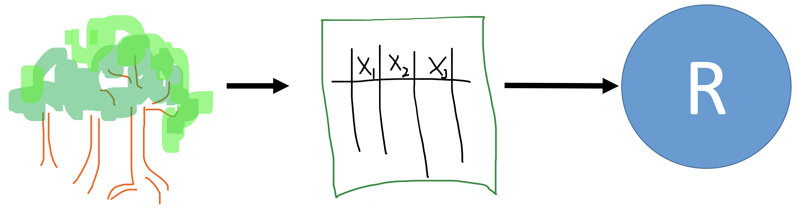 --- background-image: url(tidyr.jpeg) background-size: 100px background-position: 98% 6% # Workflow: tidy  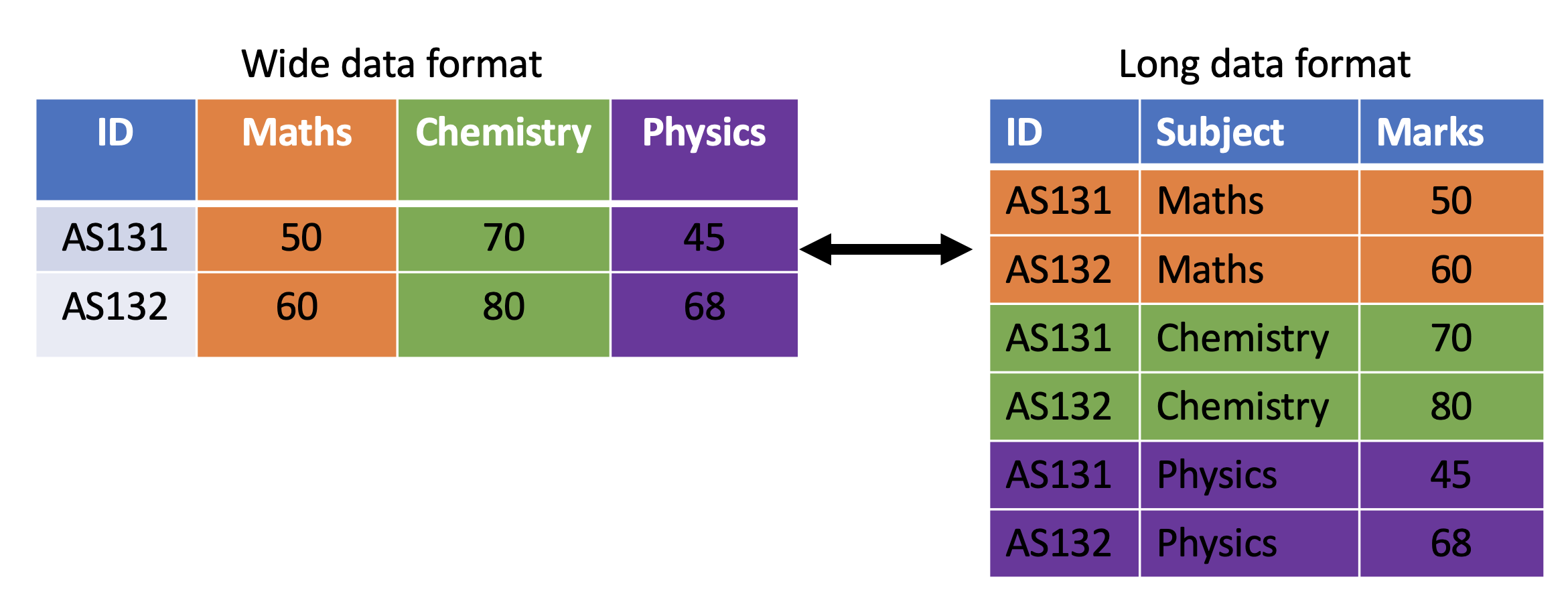 --- background-image: url(dplyr.png) background-size: 100px background-position: 98% 6% # Workflow: transform  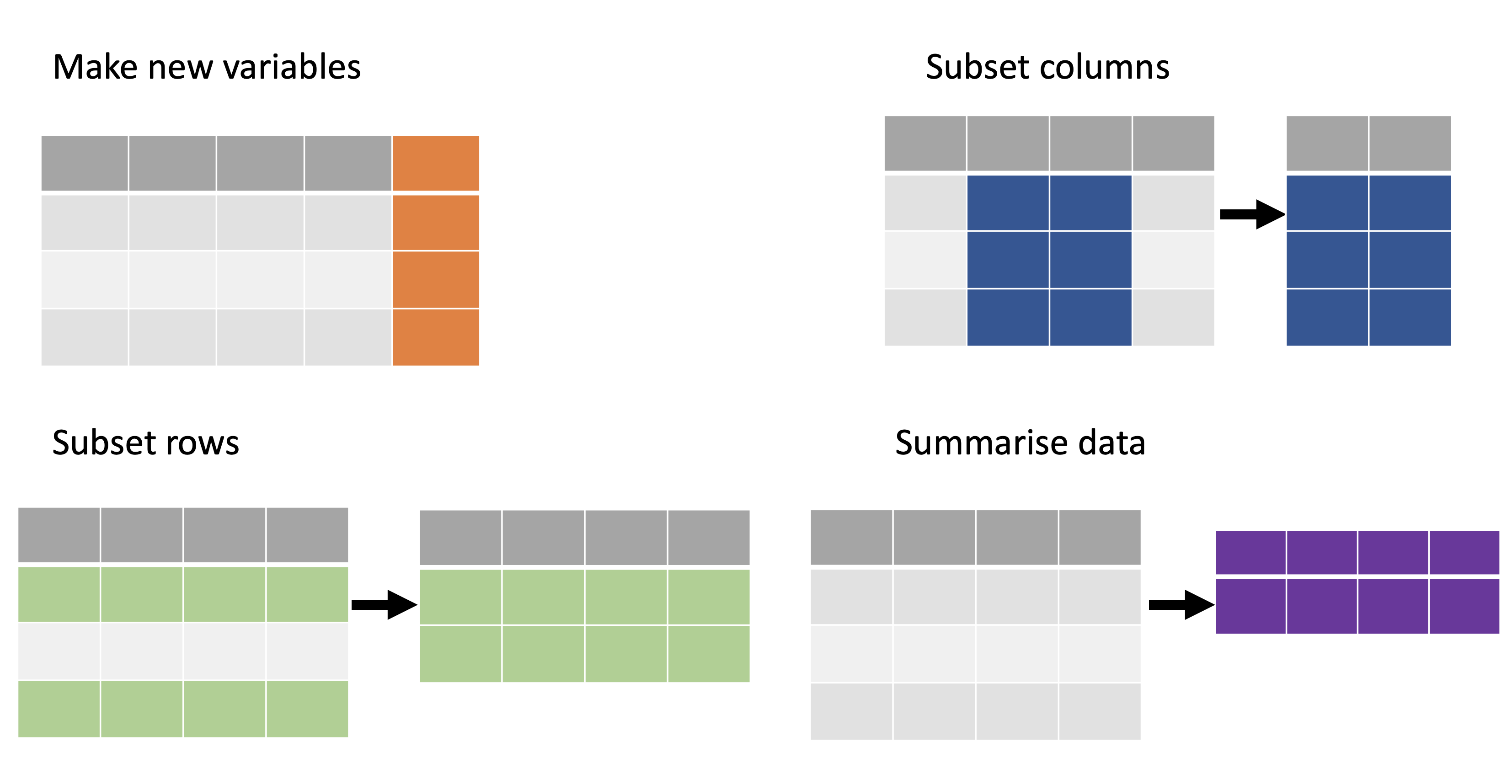 --- background-image: url(ggplot2.png) background-size: 100px background-position: 98% 6% # Workflow: visualise  ### Illustration .pull-left[ ```r library(ggplot2) ggplot(iris, aes(Sepal.Width, Sepal.Length, color=Species)) + geom_point() + theme(aspect.ratio = 1) + scale_color_manual(values = c("#1b9e77", "#d95f02", "#7570b3")) ``` ] .pull-right[ 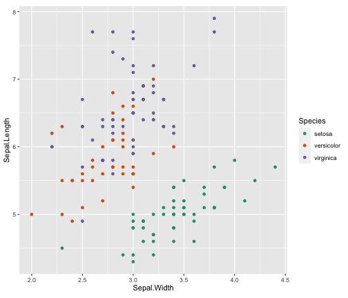<!-- --> ] --- background-image: url(purrr.png) background-size: 100px background-position: 98% 6% # Workflow: model  ## Illustration: Apply a linear model to each group ```r nested_iris <- group_by(iris, Species) %>% nest() fit_model <- function(df) lm(Sepal.Length ~ Sepal.Width, data = df) nested_iris <- nested_iris %>% mutate(model = map(data, fit_model)) nested_iris$model[[1]] # To print other two models nested_iris$model[[2]] nested_iris$model[[3]] ``` ``` Call: lm(formula = Sepal.Length ~ Sepal.Width, data = df) Coefficients: (Intercept) Sepal.Width 2.6390 0.6905 ``` --- # Workflow: communicate  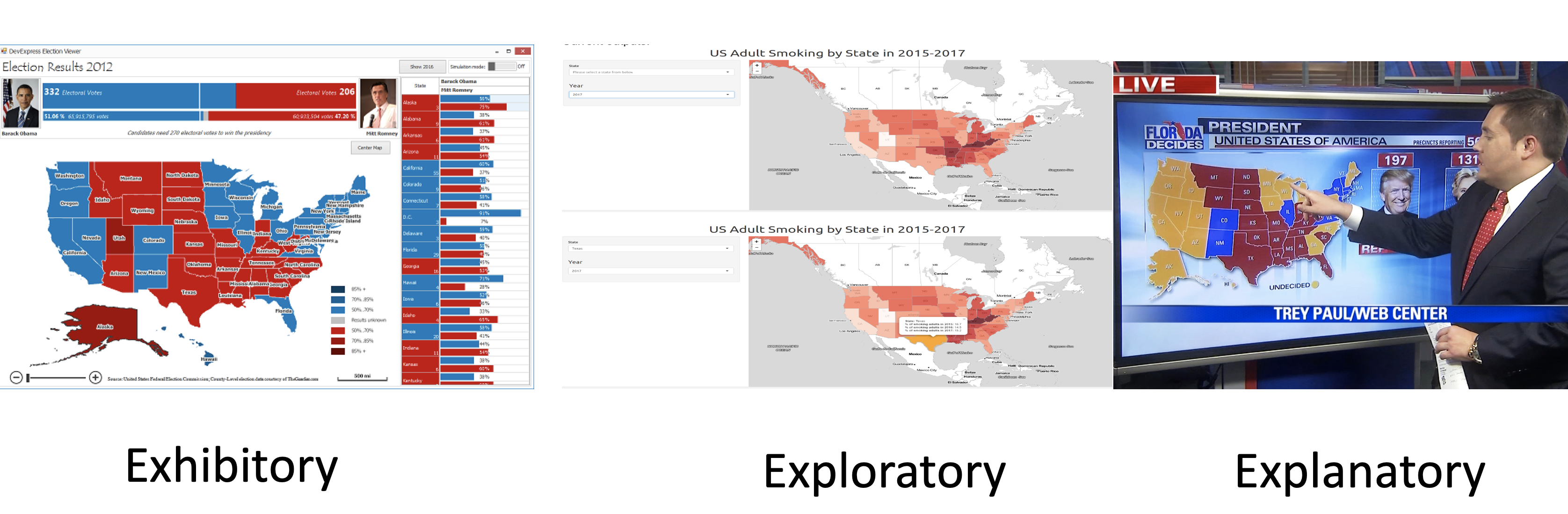 --- background-image: url(tidyvflowpkg.png) background-size: contain background-position: center # Workflow: R packages --- class: duke-softblue, middle, center # 1. Tibble # 2. Factor # 3. Pipe --- class: duke-orange, middle, center # Tibble  --- background-image: url(tibble.png) background-size: 100px background-position: 98% 6% # Tibble - Tibbles are data frames. - A modern re-imagining of data frames. # Create a tibble ```r library(tidyverse) # library(tibble) first.tbl <- tibble(height = c(150, 200, 160), weight = c(45, 60, 51)) first.tbl ``` ``` # A tibble: 3 x 2 height weight <dbl> <dbl> 1 150 45 2 200 60 3 160 51 ``` ```r class(first.tbl) ``` ``` [1] "tbl_df" "tbl" "data.frame" ``` --- # Convert an existing dataframe to a tibble ```r as_tibble(iris) ``` ``` # A tibble: 150 x 5 Sepal.Length Sepal.Width Petal.Length Petal.Width Species <dbl> <dbl> <dbl> <dbl> <fct> 1 5.1 3.5 1.4 0.2 setosa 2 4.9 3 1.4 0.2 setosa 3 4.7 3.2 1.3 0.2 setosa 4 4.6 3.1 1.5 0.2 setosa 5 5 3.6 1.4 0.2 setosa 6 5.4 3.9 1.7 0.4 setosa 7 4.6 3.4 1.4 0.3 setosa 8 5 3.4 1.5 0.2 setosa 9 4.4 2.9 1.4 0.2 setosa 10 4.9 3.1 1.5 0.1 setosa # … with 140 more rows ``` --- # Convert a tibble to a dataframe ```r first.tbl <- tibble(height = c(150, 200, 160), weight = c(45, 60, 51)) class(first.tbl) ``` ``` [1] "tbl_df" "tbl" "data.frame" ``` ```r first.tbl.df <- as.data.frame(first.tbl) class(first.tbl.df) ``` ``` [1] "data.frame" ``` --- # tibble vs. data.frame - Output **tibble** ```r first.tbl <- tibble(height = c(150, 200, 160), weight = c(45, 60, 51)) first.tbl ``` ``` # A tibble: 3 x 2 height weight <dbl> <dbl> 1 150 45 2 200 60 3 160 51 ``` **data.frame** ```r dataframe <- data.frame(height = c(150, 200, 160), weight = c(45, 60, 51)) dataframe ``` ``` height weight 1 150 45 2 200 60 3 160 51 ``` --- # tibble vs data.frame (cont.) - You can create new variables that are functions of existing variables. **tibble** ```r first.tbl <- tibble(height = c(150, 200, 160), weight = c(45, 60, 51), bmi = (weight)/height^2) first.tbl ``` ``` # A tibble: 3 x 3 height weight bmi <dbl> <dbl> <dbl> 1 150 45 0.002 2 200 60 0.0015 3 160 51 0.00199 ``` **data.frame** ```r df <- data.frame(height = c(150, 200, 160), weight = c(45, 60, 51), bmi = (weight)/height^2) # Not working ``` You will get an error message <span style="color:red">`Error in data.frame(height = c(150, 200, 160), weight = c(45, 60, 51), : object 'height' not found.`</span> --- # tibble vs data.frame (cont.) With `data.frame` this is how we should create a new variable from the existing columns. ```r df <- data.frame(height = c(150, 200, 160), weight = c(45, 60, 51)) df$bmi <- (df$weight)/(df$height^2) df ``` ``` height weight bmi 1 150 45 0.002000000 2 200 60 0.001500000 3 160 51 0.001992188 ``` --- # tibble vs data.frame (cont.) - In contrast to data frames, the variable names in tibbles can contain spaces. **Example 1** ```r tbl <- tibble(`patient id` = c(1, 2, 3)) tbl ``` ``` # A tibble: 3 x 1 `patient id` <dbl> 1 1 2 2 3 3 ``` ```r df <- data.frame(`patient id` = c(1, 2, 3)) df ``` ``` patient.id 1 1 2 2 3 3 ``` --- # tibble vs data.frame (cont.) - In contrast to data frames, the variable names in tibbles can start with a number. ```r tbl <- tibble(`1var` = c(1, 2, 3)) tbl ``` ``` # A tibble: 3 x 1 `1var` <dbl> 1 1 2 2 3 3 ``` ```r df <- data.frame(`1var` = c(1, 2, 3)) df ``` ``` X1var 1 1 2 2 3 3 ``` In general, tibbles do not change the names of input variables and do not use row names. --- # tibble vs data.frame (cont.) A tibble can have columns that are lists. ```r tbl <- tibble (x = 1:3, y = list(1:3, 1:4, 1:10)) tbl ``` ``` # A tibble: 3 x 2 x y <int> <list> 1 1 <int [3]> 2 2 <int [4]> 3 3 <int [10]> ``` This feature is not available in `data.frame`. If we try to do this with a traditional data frame we get an error. ```r df <- data.frame(x = 1:3, y = list(1:3, 1:4, 1:10)) ## Not working, error ``` <span style="color:red">`Error in (function (..., row.names = NULL, check.rows = FALSE, check.names = TRUE, : arguments imply differing number of rows: 3, 4, 10`</span> --- # Subsetting: tibble vs data.frame **Subsetting single columns:** .pull-left[ ## data frame ```r df <- data.frame(x = 1:3, yz = c(10, 20, 30)) df ``` ``` x yz 1 1 10 2 2 20 3 3 30 ``` ```r df[, "x"] ``` ``` [1] 1 2 3 ``` ```r df[, "x", drop=FALSE] ``` ``` x 1 1 2 2 3 3 ``` ] .pull-right[ ## tibble ```r tbl <- tibble(x = 1:3, yz = c(10, 20, 30)) tbl ``` ``` # A tibble: 3 x 2 x yz <int> <dbl> 1 1 10 2 2 20 3 3 30 ``` ```r tbl[, "x"] ``` ``` # A tibble: 3 x 1 x <int> 1 1 2 2 3 3 ``` ] --- **Subsetting single columns (cont):** .pull-left[ ## tibble ```r tbl <- tibble(x = 1:3, yz = c(10, 20, 30)) tbl ``` ``` # A tibble: 3 x 2 x yz <int> <dbl> 1 1 10 2 2 20 3 3 30 ``` ```r tbl[, "x"] ``` ``` # A tibble: 3 x 1 x <int> 1 1 2 2 3 3 ``` ] .pull-right[ ```r # Method 1 tbl[, "x", drop = TRUE] ``` ``` [1] 1 2 3 ``` ```r # Method 2 as.data.frame(tbl)[, "x"] ``` ``` [1] 1 2 3 ``` ] --- # Subsetting single rows with the drop argument .pull-left[ ## dataframe ```r df[1, , drop = TRUE] ``` ``` $x [1] 1 $yz [1] 10 ``` ] .pull-right[ ## tibble ```r tbl[1, , drop = TRUE] ``` ``` # A tibble: 1 x 2 x yz <int> <dbl> 1 1 10 ``` ```r as.list(tbl[1, ]) ``` ``` $x [1] 1 $yz [1] 10 ``` ] --- # Accessing non-existent columns .pull-left[ ## dataframe ```r df$y ``` ``` [1] 10 20 30 ``` ```r df[["y", exact = FALSE]] ``` ``` [1] 10 20 30 ``` ] .pull-right[ ## tibble ```r tbl$y ``` ``` Warning: Unknown or uninitialised column: `y`. ``` ``` NULL ``` ```r tbl[["y", exact = FALSE]] ``` ``` Warning: `exact` ignored. ``` ``` NULL ``` ] --- ## Functions work with both tibbles and dataframes ```r names(), colnames(), rownames(), ncol(), nrow(), length() # length of the underlying list ``` .pull-left[ ```r tb <- tibble(a = 1:3) names(tb) ``` ``` [1] "a" ``` ```r colnames(tb) ``` ``` [1] "a" ``` ```r rownames(tb) ``` ``` [1] "1" "2" "3" ``` ```r nrow(tb); ncol(tb); length(tb) ``` ``` [1] 3 ``` ``` [1] 1 ``` ``` [1] 1 ``` ] .pull-right[ ```r df <- data.frame(a = 1:3) names(df) ``` ``` [1] "a" ``` ```r colnames(df) ``` ``` [1] "a" ``` ```r rownames(df) ``` ``` [1] "1" "2" "3" ``` ```r nrow(df); ncol(df); length(df) ``` ``` [1] 3 ``` ``` [1] 1 ``` ``` [1] 1 ``` ] --- However, when using tibble, we can use some additional commands ```r is.tibble(tb) ``` ``` Warning: `is.tibble()` is deprecated as of tibble 2.0.0. Please use `is_tibble()` instead. This warning is displayed once every 8 hours. Call `lifecycle::last_warnings()` to see where this warning was generated. ``` ``` [1] TRUE ``` ```r is_tibble(tb) # is.tibble()` is deprecated as of tibble 2.0.0, Please use `is_tibble()` instead of is.tibble ``` ``` [1] TRUE ``` ```r glimpse(tb) ``` ``` Rows: 3 Columns: 1 $ a <int> 1, 2, 3 ``` --- class: duke-orange, middle, center # Factors --- # Factors - A vector that is used to store categorical variables. - It can only contain predefined values. Hence, factors are useful when you know the possible values a variable may take. ## Creating a factor vector ```r grades <- factor(c("A", "A", "A", "C", "B")) grades ``` ``` [1] A A A C B Levels: A B C ``` -- Now let's check the class type ```r class(grades) # It's a factor ``` ``` [1] "factor" ``` -- To obtain all levels ```r levels(grades) ``` ``` [1] "A" "B" "C" ``` --- ## Creating a factor vector (cont) - With factors all possible values of the variables can be defined under levels. ```r grade_factor_vctr <- factor(c("A", "D", "A", "C", "B"), levels = c("A", "B", "C", "D", "E")) grade_factor_vctr ``` ``` [1] A D A C B Levels: A B C D E ``` ```r levels(grade_factor_vctr) ``` ``` [1] "A" "B" "C" "D" "E" ``` ```r class(levels(grade_factor_vctr)) ``` ``` [1] "character" ``` --- # Character vector vs Factor - Observe the differences in outputs. Factor prints all possible levels of the variable. **Character vector** ```r grade_character_vctr <- c("A", "D", "A", "C", "B") grade_character_vctr ``` ``` [1] "A" "D" "A" "C" "B" ``` **Factor vector** ```r grade_factor_vctr <- factor(c("A", "D", "A", "C", "B"), levels = c("A", "B", "C", "D", "E")) grade_factor_vctr ``` ``` [1] A D A C B Levels: A B C D E ``` --- # Character vector vs Factor (cont.) - Factors behave like character vectors but they are actually integers. **Character vector** ```r typeof(grade_character_vctr) ``` ``` [1] "character" ``` **Factor vector** ```r typeof(grade_factor_vctr) ``` ``` [1] "integer" ``` --- # Character vector vs Factor (cont.) - Let's create a contingency table with `table` function. **Character vector output with table function** ```r grade_character_vctr <- c("A", "D", "A", "C", "B") table(grade_character_vctr) ``` ``` grade_character_vctr A B C D 2 1 1 1 ``` **Factor vector (with levels) output with table function** ```r grade_factor_vctr <- factor(c("A", "D", "A", "C", "B"), levels = c("A", "B", "C", "D", "E")) table(grade_factor_vctr) ``` ``` grade_factor_vctr A B C D E 2 1 1 1 0 ``` - Output corresponds to factor prints counts for all possible levels of the variable. Hence, with factors it is obvious when some levels contain no observations. --- # Character vector vs Factor (cont.) - With factors you can't use values that are not listed in the levels, but with character vectors there is no such restrictions. **Character vector** ```r grade_character_vctr[2] <- "A+" grade_character_vctr ``` ``` [1] "A" "A+" "A" "C" "B" ``` **Factor vector** ```r grade_factor_vctr[2] <- "A+" ``` ``` Warning in `[<-.factor`(`*tmp*`, 2, value = "A+"): invalid factor level, NA generated ``` ```r grade_factor_vctr ``` ``` [1] A <NA> A C B Levels: A B C D E ``` --- # Modify factor levels This our factor ```r grade_factor_vctr ``` ``` [1] A <NA> A C B Levels: A B C D E ``` ## Change labels ```r levels(grade_factor_vctr) <- c("Excellent", "Good", "Average", "Poor", "Fail") grade_factor_vctr ``` ``` [1] Excellent <NA> Excellent Average Good Levels: Excellent Good Average Poor Fail ``` ## Reverse the level arrangement ```r levels(grade_factor_vctr) <- rev(levels(grade_factor_vctr)) grade_factor_vctr ``` ``` [1] Fail <NA> Fail Average Poor Levels: Fail Poor Average Good Excellent ``` --- # Order of factor levels **Default order of levels** ```r fv1 <- factor(c("D","E","E","A", "B", "C")) fv1 ``` ``` [1] D E E A B C Levels: A B C D E ``` ```r fv2 <- factor(c("1T","2T","3A","4A", "5A", "6B", "3A")) fv2 ``` ``` [1] 1T 2T 3A 4A 5A 6B 3A Levels: 1T 2T 3A 4A 5A 6B ``` -- ```r qplot(fv2, geom = "bar") ``` 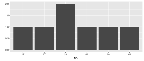<!-- --> --- # Order of factor levels (cont.) You can change the order of levels ```r fv2 <- factor(c("1T","2T","3A","4A", "5A", "6B", "3A"), levels = c("3A", "4A", "5A", "6B", "1T", "2T")) fv2 ``` ``` [1] 1T 2T 3A 4A 5A 6B 3A Levels: 3A 4A 5A 6B 1T 2T ``` ```r qplot(fv2, geom = "bar") ``` 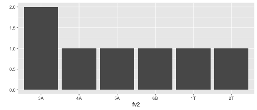<!-- --> --- Note that tibbles do not change the types of input variables (e.g., strings are not converted to factors by default). ```r tbl <- tibble(x1 = c("setosa", "versicolor", "virginica", "setosa")) tbl ``` ``` # A tibble: 4 x 1 x1 <chr> 1 setosa 2 versicolor 3 virginica 4 setosa ``` ```r df <- data.frame(x1 = c("setosa", "versicolor", "virginica", "setosa")) df ``` ``` x1 1 setosa 2 versicolor 3 virginica 4 setosa ``` ```r class(df$x1) ``` ``` [1] "character" ``` --- class: duke-orange, middle, center # Pipe operator: %>%  --- background-image: url(magrittrlogo.png) background-size: 100px background-position: 98% 6% # Pipe operator: %>% ## Required package: `magrittr` ```r install.packages("magrittr") library(magrittr) ``` ## What does it do? It takes whatever is on the left-hand-side of the pipe and makes it the first argument of whatever function is on the right-hand-side of the pipe. For instance, ```r mean(1:10) ``` ``` [1] 5.5 ``` can be written as ```r 1:10 %>% mean() ``` ``` [1] 5.5 ``` --- # Pipe operator: %>% 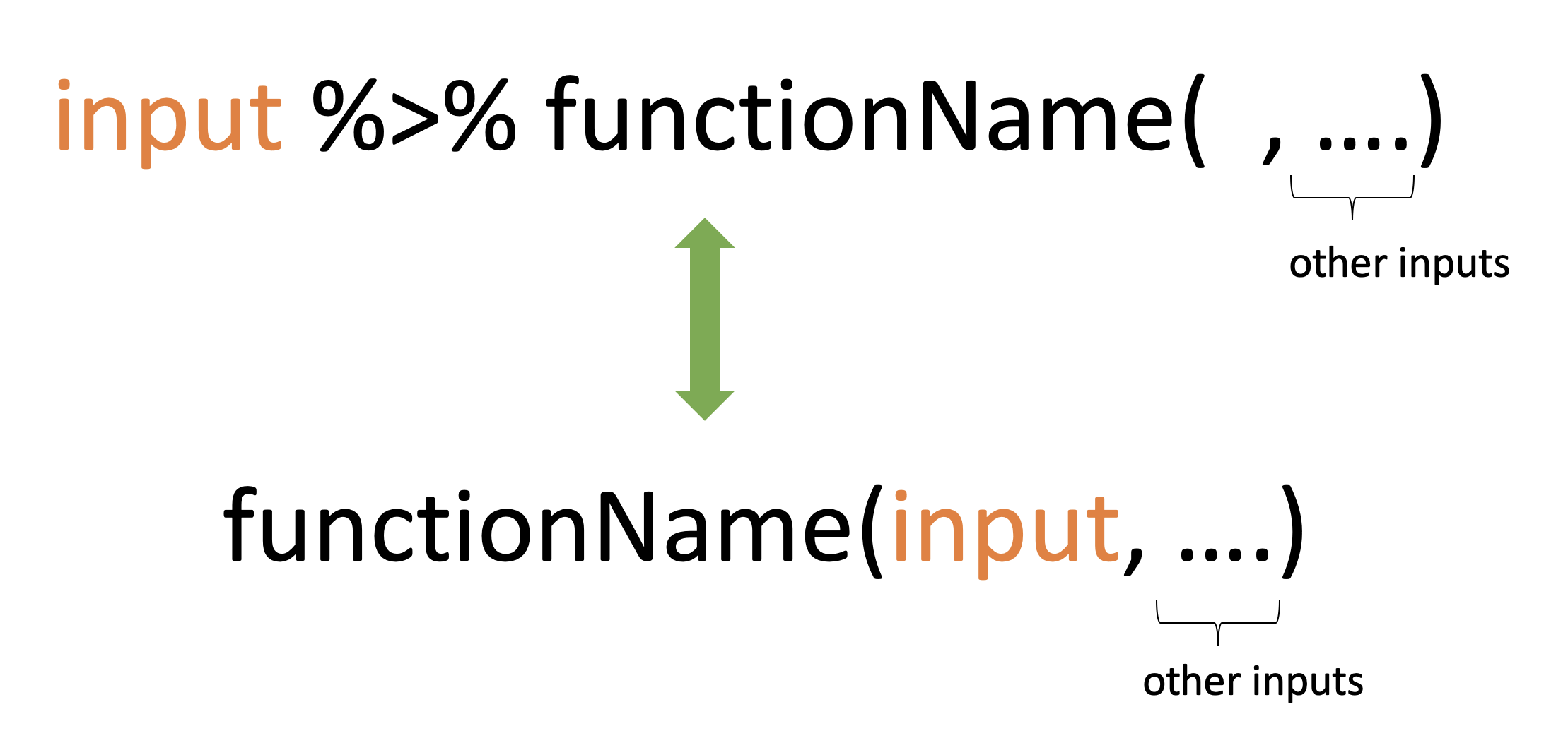 ## Illustrations 1. `x %>% f(y)` turns into `f(x, y)` 1. `x %>% f(y) %>% g(z)` turns into `g(f(x, y), z)` --- # Why %>% - This helps to make your code more readable. **Method 1: Without using pipe (hard to read)** ```r colSums(matrix(c(1, 2, 3, 4, 8, 9, 10, 12), nrow=2)) ``` ``` [1] 3 7 17 22 ``` **Method 2: Using pipe (easy to read)** ```r c(1, 2, 3, 4, 8, 9, 10, 12) %>% matrix( , nrow = 2) %>% colSums() ``` ``` [1] 3 7 17 22 ``` or ```r c(1, 2, 3, 4, 8, 9, 10, 12) %>% matrix(nrow = 2) %>% # remove comma colSums() ``` ``` [1] 3 7 17 22 ``` --- # Rules ```r library(tidyverse) # to use as_tibble library(magrittr) # to use %>% df <- data.frame(x1 = 1:3, x2 = 4:6) ``` .pull-left[ **Rule 1** ```r head(df) df %>% head() ``` ``` x1 x2 1 1 4 2 2 5 3 3 6 ``` **Rule 2** ```r head(df, n = 2) df %>% head(n = 2) ``` ``` x1 x2 1 1 4 2 2 5 ``` ] .pull-right[ **Rule 3** ```r head(df, n = 2) 2 %>% head(df, n = .) ``` ``` x1 x2 1 1 4 2 2 5 ``` **Rule 4** ```r head(as_tibble(df), n = 2) df %>% as_tibble() %>% head(n = 2) ``` ``` # A tibble: 2 x 2 x1 x2 <int> <int> 1 1 4 2 2 5 ``` ] --- # Rules (cont.) **Rule 5: subsetting** ```r df$x1 df %>% .$x1 ``` ``` [1] 1 2 3 ``` or ```r df[["x1"]] df %>% .[["x1"]] ``` ``` [1] 1 2 3 ``` or ```r df[[1]] df %>% .[[1]] ``` ``` [1] 1 2 3 ``` --- # Offline reading materials Type the following codes to see more examples: ```r vignette("magrittr") vignette("tibble") ``` --- class: center, middle Slides available at: hellor.netlify.com All rights reserved by [Thiyanga S. Talagala](https://thiyanga.netlify.com/)